Simulating Channel Fluid Mixing in Taichi

(2026/09/23)

This is an extension of my earlier experiment on simulating a lid-driven cavity in Taichi. Previously, I primarily focused on understanding some theory on how fluid simulations were implemented, specifically with how to deal with the NS equation and the Chorin projection method. This time, I attempt to extend it for a task more suited to me as an engineering student.

Simulation Showcase

The inspiration for this simulation is the idea of microreactors. In scaling-up certain reactions, heat transfer becomes a crucial step, and one way to address this is to react the chemicals in microchannels, where the area-to-volume ratio is quite large. Operating under continuous flow in this small domains, however, results in the fluid behaving laminarly (similar to a system with low Re), which can make it hard to mix reactants and achieve high percent yield.

In big reactors, it is easy to use big mixers to solve this issue. But in a small microchannel, we must instead utilize obstacle geometries (known as passive mixers) and vary the operating parameters (e.g., flowrate) to intrinsically encourage mixing. This is what I wanted to explore with this simulation. For full details of the updates to the code I made since last time, check the Technical Details.

Test 1: Behaviors at different Re

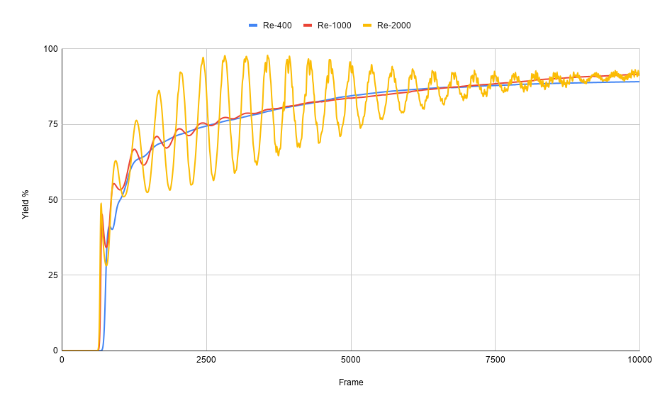
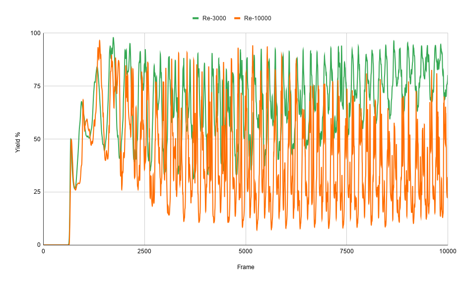
I first validated the simulation by testing how it responds when I varied the Reynold’s number of the fluid. I tested five different Re values: 400, 1000, 2000, 3000, 10000 while keeping the rest of the parameters constant. In this test, I used a series of staggered semicircles for the obstacles (“geometry 1”). The yield percent at the outlet tracked across frames (~time) are shown in the graphs below.

Laminar regime (Re = 400, 1000, 2000)

Turbulent regime (Re = 3000, 10000)

Note: The other parameters held constant are u_inlet = 0.1, k = 1.0e4, D = 0.0001

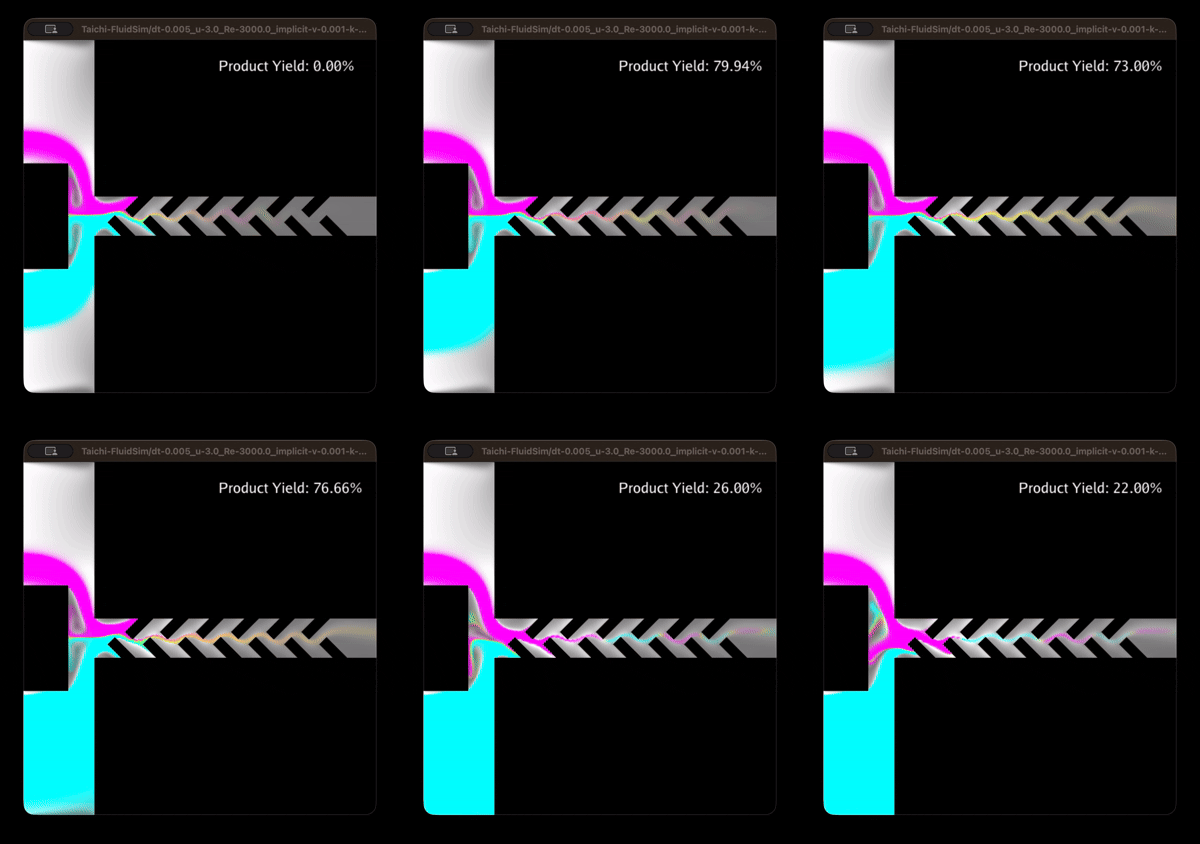
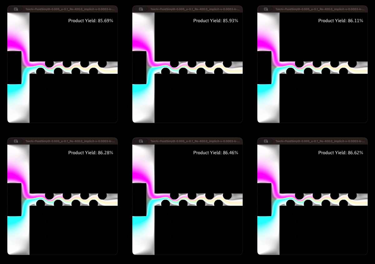
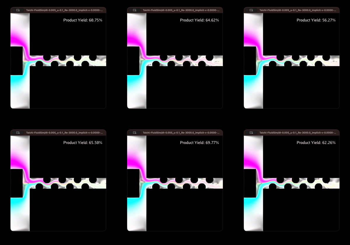
As expected, we see the general trend of increasing “volatility” as we increase the Reynold’s number of the fluid. If we take a look at the simulations (below), we can explain why we get this pattern in the yields of different Re values. Looking at the flow of Re = 3000, we can notice the outlet composition alternating between the product (in yellow) and the ‘leaking’, unreacted reactants (in magenta and cyan). This generates instances of low and high recorded yield, resulting in the oscillating graph. Laminar flow (such as Re = 400) meanwhile shows more consistent composition at the outlet, which explains the more stable curve through time.

Re = 400 snippet

Re = 3000 snippet

Test 2: Varying inlet speed u_inlet

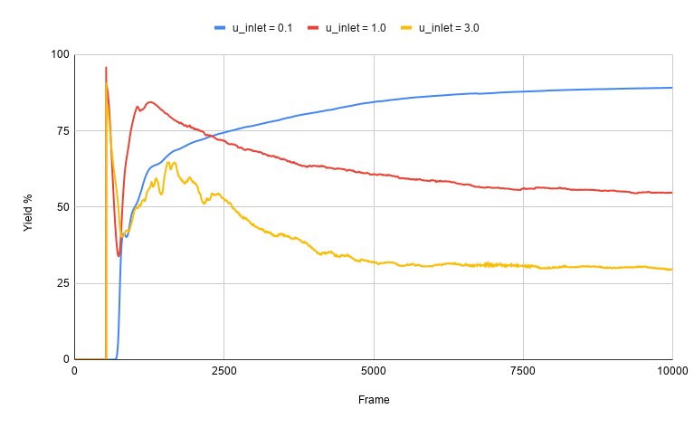
Aside from the mixing geometry, the other prominent factor contributing to the degree of mixing of the reactants (and thus the reaction progress/yield) would be diffusion. This, however, requires residence time in the channel, which becomes shorter as the flow speed increases. Consequently, we expect the yield percentage to decrease at higher fluid velocities.

If we look at the graph below, this is exactly what we get when we vary the u_inlet in a simulation for laminar flows (Re = 400). While there is an early, initial spike in yield percentage for high velocities, the behaviors at steady-state (roughly beyond frame 7000) show the highest yield for the lowest speed (u_inlet = 0.1).

Yield percentage of different inlet speeds

Test 3: Varying obstacle geometry

Finally, we can try comparing what happens when we change the design of the obstacles that are meant to act as passive mixers. Aside from the geometry_1 used in Tests 1 and 2, I also implemented a geometry_2 featuring staggered tilted rectangles. Setting Re = 400 and u_inlet = 0.1, we get the following yield percentage curves:

Yield percentage of different geometries

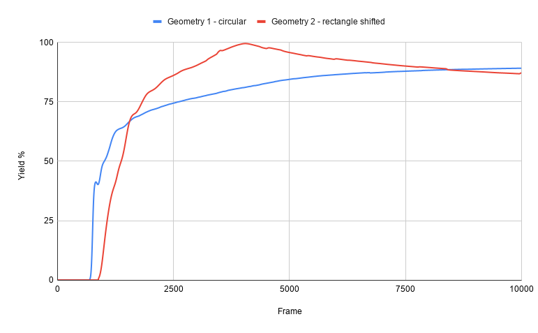
Over the 10,000 frame period, geometry_2 slightly edges out with a total yield* of 78.89% versus the geometry_1 with 74.95%. However, we do notice that the 1st geometry stabilizes at a slightly higher yield percent, which suggests it might be more efficient if we operate for much longer.

* total yield = (area under the yield curve) / (rectangular area of 100% * 10,000 frames)

Geometry 1 flow

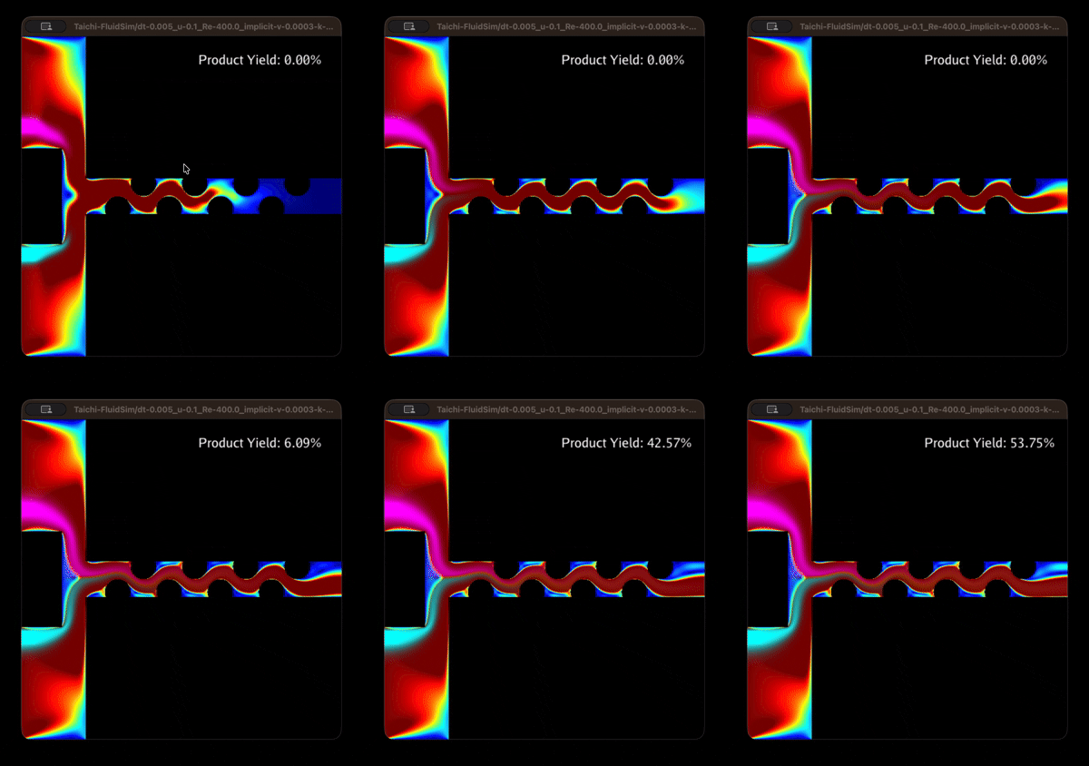
Geometry 2 flow

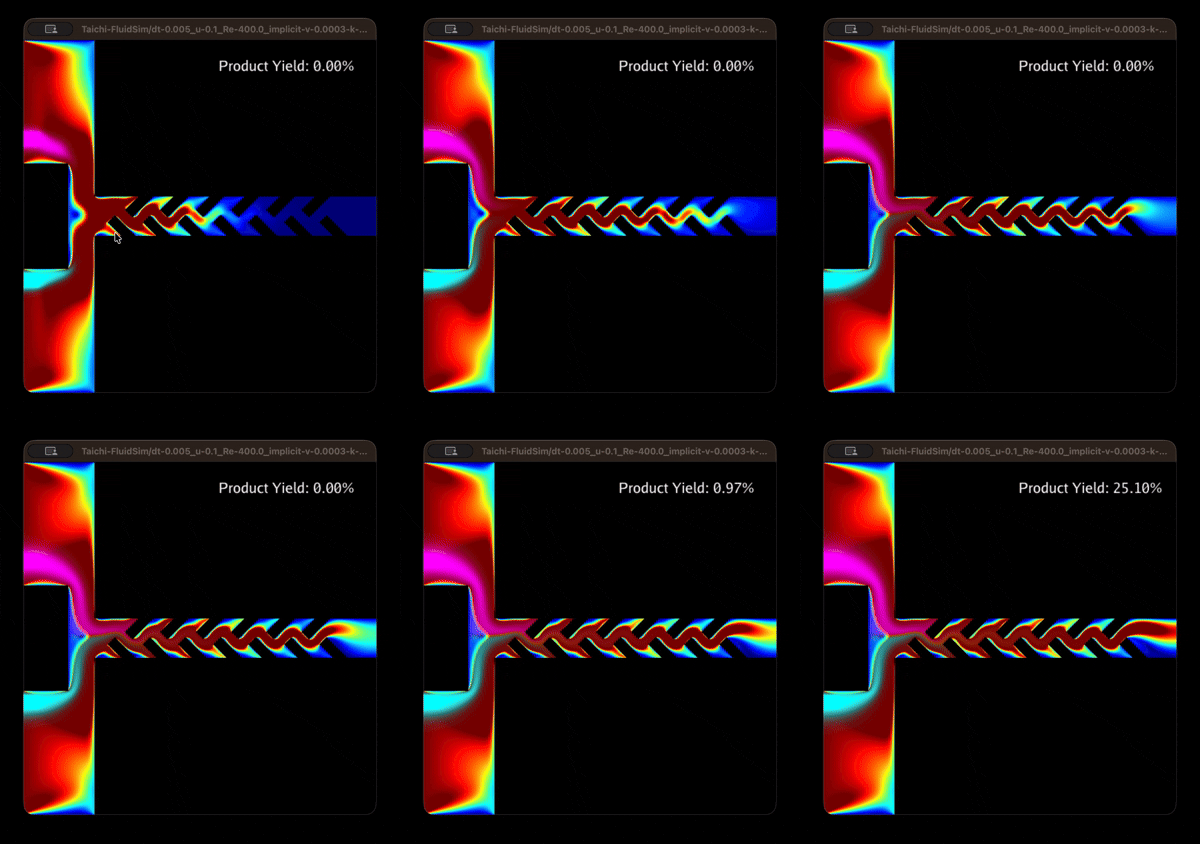
We can also notice from the simulation flows that geometry_1 has an overall larger throughput since the curved geometry is less a bottleneck for fluid flow and outlet velocity. In terms of total product flux (t.p.f.) over the same 10,000-frame sampling period, the circular obstacles has a t.p.f. of ~12,000, whereas the tilted rectangles have a t.p.f. of only ~900.

What works best?

Looking at the results so far, it would seem that we get the best yield when we have a fluid moving laminarly (low Re), slowly (low u_inlet), and with a sharp passive mixer like geometry_2.

However, this only optimizes for yield percentage (a.k.a. efficiency), and not necessarily total throughput. If we were to optimize for total product flux, we would in fact want higher speeds, at the cost of conversion rate. For example, while u_inlet = 0.1(~74%) shows significantly higher yield than u_inlet = 3.0 (~36%) in Test 2, the total product flux for the faster speed case (t.p.f. = ~42000) is more than 3 times that of the slower inlet flow (t.p.f. = ~12000). In a real-world setting, the higher throughput would be more favorable, although of course other factors (e.g., separation processes) should also be accounted for.

Technical Details

I also made another set of notes this time around. Similar to last time, it contains a bit more detail on the exact equations used for the simulation.

The change I made can be briefly outlined into 4 points:

1. Allowing for mass transport. The dye representing the chemicals is modeled in simulation as a multicomponent scalar field $C$. It is governed by the following incompressible advection equation, accounting for molecular diffusion with constant $D$:

$$\frac{\partial C}{\partial t} + \bm{u} \cdot \nabla C = D \nabla^{2} C$$

Each component in $C$ represents a different dye, i.e., for a three-dye system consisting of reactants A and B, and product C, we have:

$$C = \begin{pmatrix} C_A \\ C_B \\ C_C \end{pmatrix}$$

Now, when solving this numerically, I employed the MacCormack method for higher order advection, which helps lessen the artificial diffusion generated by the numerical errors of first-order approximations.

2. Custom boundary conditions geometries. The passive mixers are then modeled using functions that accept a position $(i,j)$ and outputs a boolean on whether it corresponds to a obstacle coordinate or not. Check the code for how I implemented the base functions for circular and rectangular obstacles.

3. Allowing for reactions between different dyes. Suppose the dyes react according to $A+B \rightarrow C$, with the rate equation,

$$\frac{dC_C}{dt} = k C_A C_B .$$

Accounting for limiting reagents, the amount of generated dye C in a cell $(i, j)$ over the time step $\delta t$ is given by:

$$\Delta C_C |_{i, j} = \min{(k C_A C_B \delta t, \min{(C_A, C_B)})} |_{i, j}$$

4. Measuring output yield. As a rough measure on the performance of the passive mixers, we can measure the reaction yield based on the outgoing flux of the different dyes. Specifically, we define this yield to be the ratio of the dye C flux to the total flux near the right wall outlet ($i=N-2$)

$$\% \ \text{yield} = \frac{\phi_C}{\phi_{total}} = \frac{\sum_{j=0} ^N{(C_C \cdot \bm{u}_x) | _{N-2, j}}}{{\sum_{j=0} ^N{((C_A + C_B + C_C) \cdot \bm{u}_x) | _{N-2, j}}}}$$

Final Notes

I had a lot of fun exploring fluid sims, and I think I might come back to this again in the future, probably coupling other systems (e.g., charge carriers like ions) and external forces (e.g., applied voltages).