Lid-driven Cavity Simulation with Taichi

(2026/09/08)

Some preface

I took a class on vector calculus last third semester thinking all I would be doing is solving integrals and applying Stoke’s Theorem…but that was a lie.

I ended up being introduced to the Navier-Stokes equation:

$$\rho \frac{D\bm{u}}{Dt} = \rho \bm{K} - \nabla p + (\lambda + \mu)(\nabla (\nabla \cdot \bm{u})) + \mu \nabla^2 \bm{u}$$

and honestly, I have always wanted to know more about the NS equation, considering its fame (or infamy) as one of the Clay Institute’s Millenium Problems. The class was more of a off-syllabus rollercoaster on some analysis of the NS equation using results from functional analysis (like Riesz representation, Helmholtz decomposition, Lax-Milgram, etc.) with weak formulations over L2 space.

Anyways, as an engineering student, I recently thought about going back to what we went over in that class and using it as foundations for a task I have always wanted to try: fluid sims!

Simulation Showcase

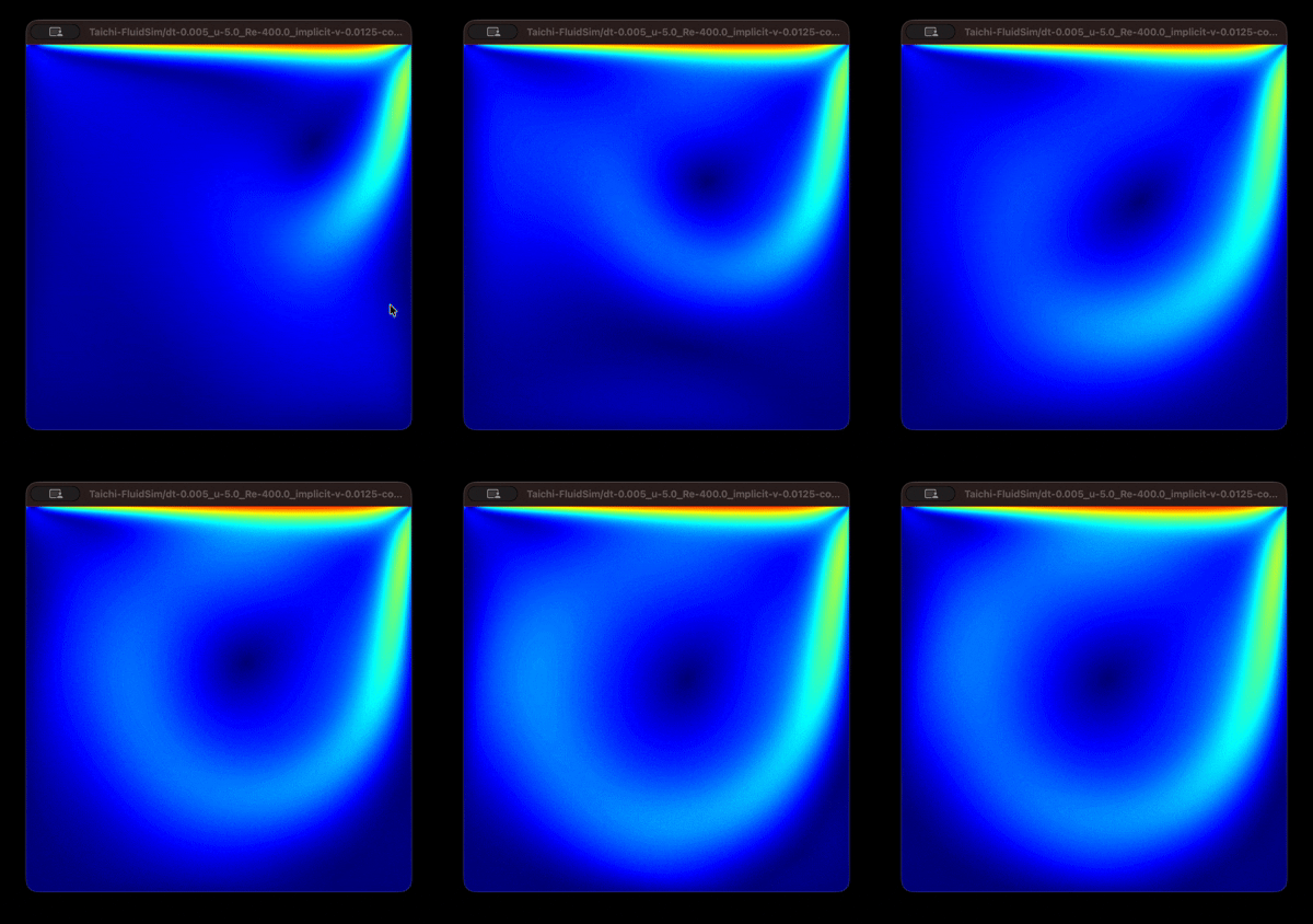
For this task, I took the Eulerian-approach to fluid simulations, i.e., using a mesh on which you track fluxes rather than individual particles. Specifically, I used a simulation method known as Chorin projection, which leverages the fact that solutions to the incompressible NS equation can be Hodge decomposed, which allows us to split the update steps into multiple manageable steps (see details below). The entire program was implemented in Python using Taichi, a useful library for running Python programs on the GPU.

Sim 1: Explicit viscosity at shorter dt

The NS equation allows us to consider the internal friction or “viscosity” in our system. Broadly speaking, we can deal with this viscosity term explicitly or implicitly. As a general rule of thumb, we can treat the explicit solution as closer to ground-truth, assuming our time step $dt$ is sufficiently small to be a stable update. Running the simulation with the explicit viscosity simulation with Reynold’s number $Re=400$ and time step $\delta t = 7 \times 10^{-5}$ produces this velocity distribution:

(Note: Warmer colors = higher fluid speed)

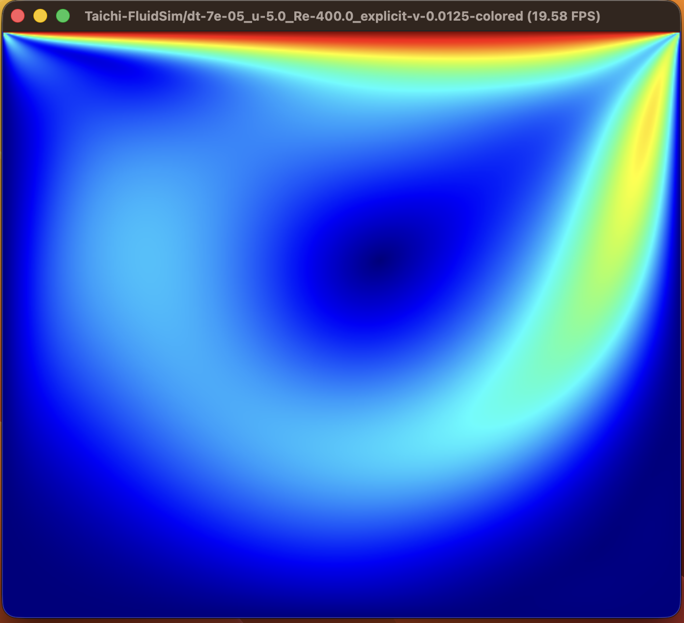
The formation of the cavity (the slow, blue circular region) is a sign that the implementation is successful. This matches closely with this reference from MIT CalculiX.

Sim 2: Implicit viscosity at longer dt

The other method for solving viscosity is to do so implicitly, or via an interative approximation. At the cost of accuracy in more minute details, you can run this simulation at a decent frame rate in real time using much longer time steps. We can see this in the simulation below, which is ran at the same $Re=400$ but this time with $\delta t = 0.005$ (nearly two orders of magnitude bigger).

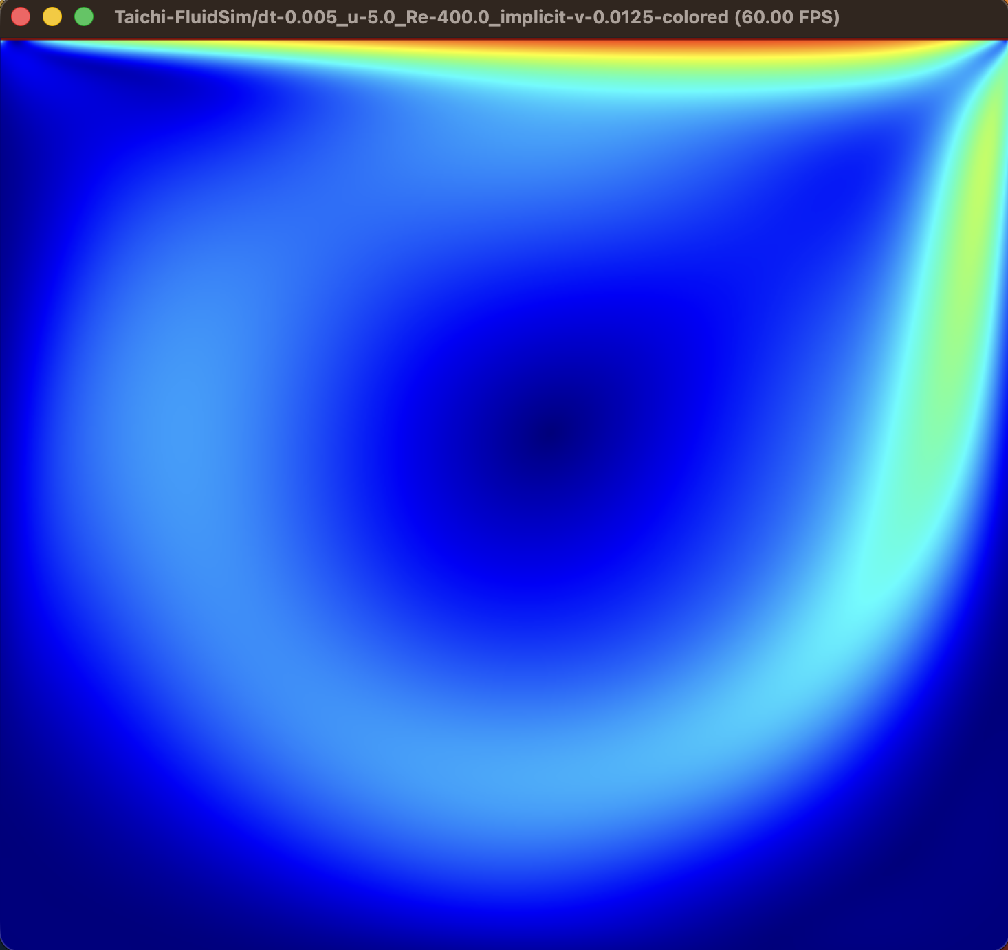
The formation of the cavity is clear, which suggests this run is acceptable. However, you can notice some differences to the previous run, particularly with the shape of the cavity this time being much more “symmetric”. This is less accurate to the real-world phenomenon in this regard.

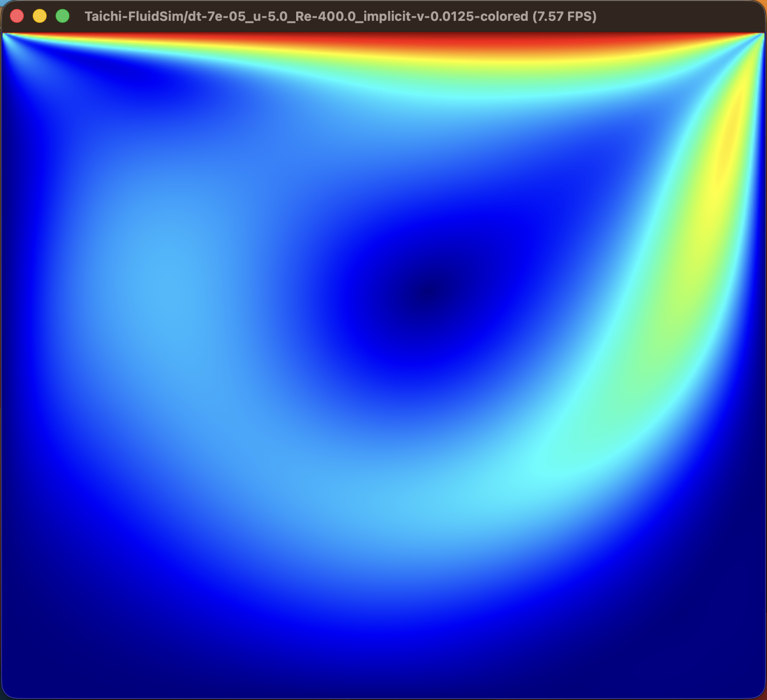
It should be noted that we can also run the implicit viscosity solver at the same short time-step of $\delta t = 7 \times 10^{-5}$, but we lose the benefit of high frame rates (it drops to less than 10 fps, as shown). From this, we can say that it is better to use the explicit solver if we are aiming for higher physical accuracy, and the implicit solver if we are instead looking for more real-time visualizations.

Technical Details

I took handwritten notes (uploaded on GDrive) as I was implementing this mini-project and trying to wrap my head around the algorithm.

As a starting point, we can begin with the incompressible NS equation (i.e., $\nabla \cdot {\bm{u}}=0$) with no external forces:

$$\frac{\partial \bm{u}}{\partial t} + (\bm{u} \cdot \nabla)\bm{u} = \frac{1}{\rho} \nabla p + \nu \nabla ^ 2 \bm{u}$$

The task is to update the velocity and static pressure fields as time progresses.

Chorin Project Method (from 1.2 of the notes)

Visualizing the velocity field by solving the above equation directly is difficult due to the coupling of both velocity and pressure updates from a single equation. As such, we instead do the update in steps:

1. Advection. We temporarily ignore the RHS, and simply update the velocity field to an intermediate $\bm{u^*}$ by solving:

$$\frac{\partial \bm{u}}{\partial t} = - (\bm{u} \cdot \nabla)\bm{u}$$

This can be implemented in a partly particle-like manner.

2. Viscosity. Next, we apply the effects of internal friction by updating to another intermediate $\bm{u^{**}}$ according to the viscosity term. This is done by solving:

$$\frac{\partial \bm{u}}{\partial t} = \nu \nabla ^ 2 \bm{u}$$

The Laplacian $\nabla ^ 2$ can be approximated like a local pooling (averaging).

3. External Forces. If there are external forces, the update will simply involve accounting for the resulting external acceleration:

$$\bm{u^{***}} := \bm{u^{**}} + \bm{a}_{ext} \delta t.$$

However, since there are no external forces in this task, we can forego this step.

4. Projection (for static pressure). Now, suppose we have a suitable pressure field $p$ that, if we apply, maintains the incompressibility condition of $\bm{u}$. Then, the final update to the velocity is simply:

$$\bm{u} := \bm{u^{***}} - \left(\frac{1}{\rho} \nabla p \right) \delta t$$

The problem now is how to find this corresponding pressure field $p$. To do this, we find the divergence of the resulting velocity field $\nabla \cdot u$, and it should be zero due to incompressibility. As such, to find the pressure field, we solve:

$$\nabla ^ 2 p = \frac{\rho}{\delta t} \nabla \cdot \bm{u^{***}}$$

This can be approximated iteratively.

Substepping

We can run multiple updates before displaying a frame so that the movements in the simulation does not take too long. This is a technique known as substepping. In the code, this is applied to the explicit viscosity solver.

Remarks

Next, I want to try extending this simulation to also account for mass transport, to simulate dye dissapation (for example). The final goal is to try to simulate different geometries and study how they mix microfluidic flows (where a laminar regime dominates).

Also, while I was writing this post I came across the ongoing developments regarding the supposed solution NS Millenium Problem, particularly on the announcement by Tristan Buckmaster and Levent Alpöge here. From what I can understand, if their proof is to be validated, this would be a groundbreaking case of AI aiding in what should still be human-directed research programmes, especially in math.