Liquid-Vapor Transitions

(2025/08/30)

Recently, I stumbled upon a 3Blue1Brown video on simulating phase change. There, Vilas Weinstein explained a powerful but relatively simple way of modeling the phase transition between liquid and vapor/gas. I was quickly interested and decided to give the implementation a shot in Python.

Simulation Showcase

Rudimentary visualizations (UI, etc.) were built through TKinter. Here’s I show a quick look at the final interactive simulations I made. To try it out for yourself, visit the repo at my GitHub and run the code locally.

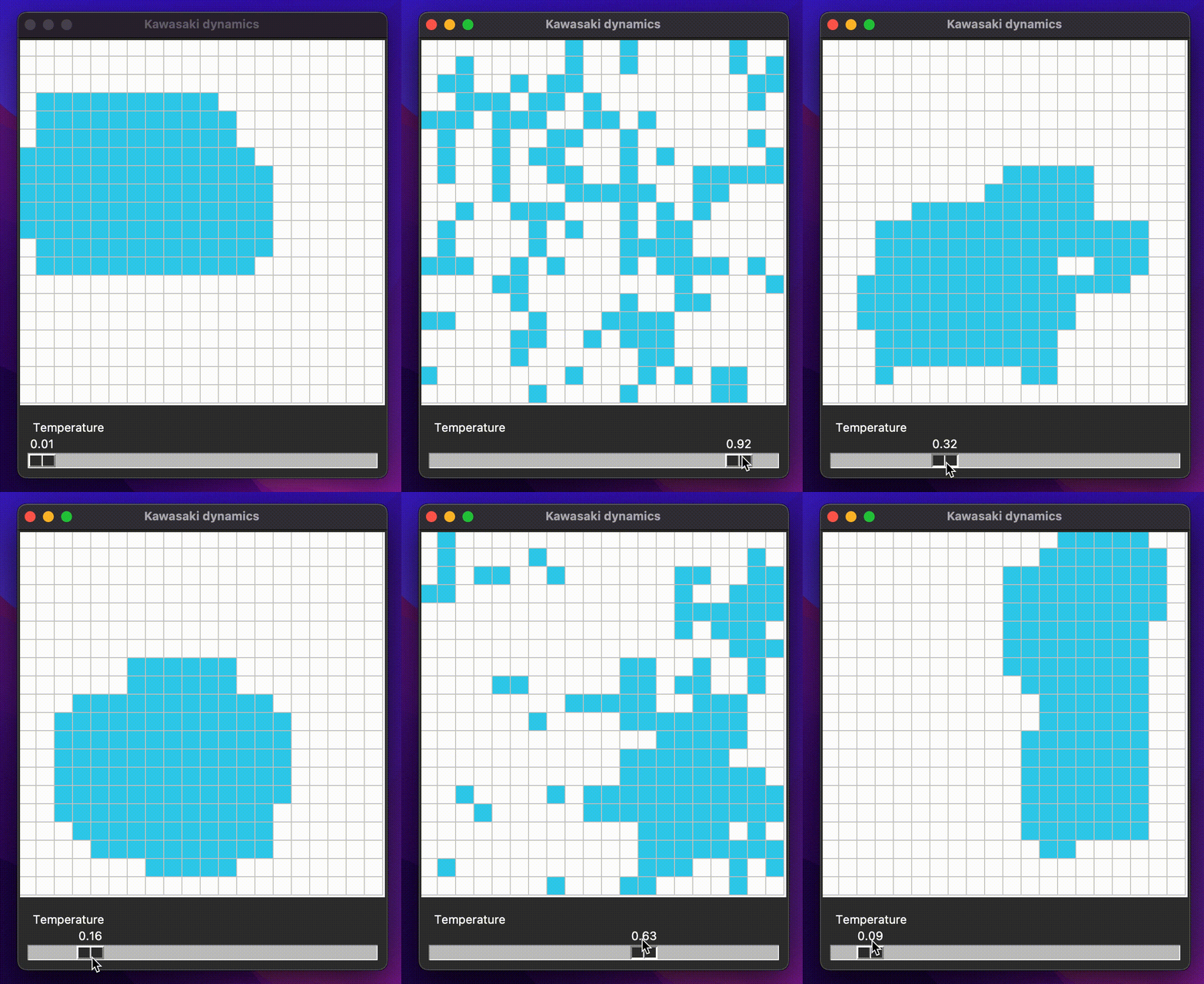
Temperature-dependence via Kawasaki dynamics

Here, the parameter you control is the temperature of the system. At low temperatures, you can notice that the molecules bundle up together into blobs—indicating a liquid phase. At higher temperatures, the molecules are more random and entropic, thereby exhibiting the gas phase.

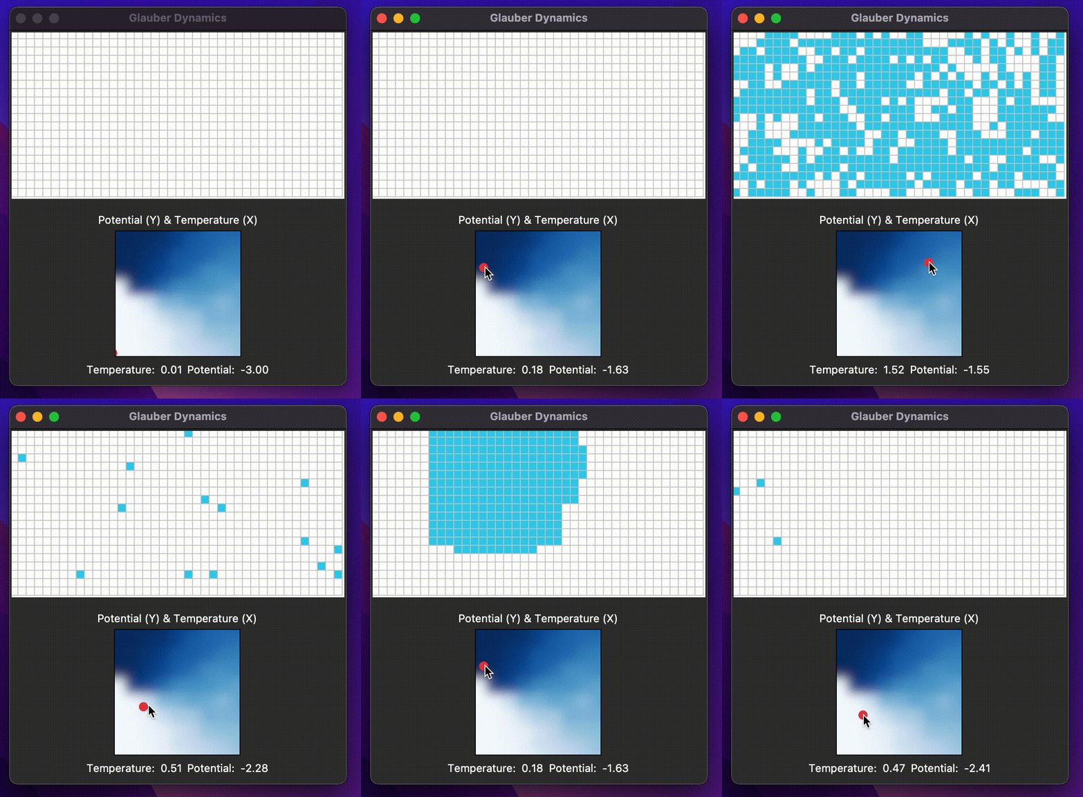
Temperature and chemical potential-dependence via Glauber dynamics

In an actual phase diagram, the two parameters are temperature and pressure. However, as explained in the 3B1B video, pressure is tricky to implement because it requires dynamically changing the volume or size of the system. Because of that, we can instead control the amount of molecules through something called the chemical potential of the system. In this implementation, you can use the 2D slider to control temperature (x-axis) and potential (y-axis).

The background of the 2D slider is actually the phase diagram I sampled from this very simulation (with a bit of blur post-processing). Blue color indicates a more liquid phase. At high temperatures (right side of the slider), the boundary between liquid and gas becomes “blurry”. This roughly models a supercritical fluid phase.

Technical Details

First of all, I highly recommend watching the 3B1B video for the amazing visualizations and intuitive explanations behind the derivation of the model. Here, I’ll try to give a gist of my implementation.

Sim. 1: Kawasaki dynamics

Consider the system to be at some temperature $T$. In this simulation, the energy $E(X)$ at some system state $X$ is modeled as the negative of the number of pairs of adjacent molecules. To propagate the simulation, the following rules are followed:

1. Randomly choose two cells $c_1$, $c_2$ in the grid, one of which is occupied by a molecule (value: 1) and the other is free (value: 0)
2. Calculate the current energy $E_0$ of the grid.
3. Flip the values of both $c_1$ and $c_2$.
4. Calculate the new energy $E_1$ of the grid.
5. Calculate the probability threshold $P$ where $P = q/(1+q)$ and

$$q = \exp{\left(\frac{E_0-E_1}{T}\right)}$$

6. Generate a random real number $s\in[0,1]$. If $s \geq P$, revert back the values of $c_1$ and $c_2$ (i.e., flip once more)

Sim. 2: Glauber dynamics

Consider the system to be at some temperature $T$ and chemical potential $C$. Here, the energy $E_G(X)$ is modeled as $E(X)-C \cdot N(X)$, where $E(X)$ is the same as in Kawasaki dynamics, and $N(X)$ simply refers to the number of molecules at some state $X$. Then, it iterates by:

1. Randomly choose one cell $c_1$ from the grid.
2. Calculate the current energy $E_0$ of the grid.
3. Calculate the final energy $E_1$ of the grid if the value of $c_1$ was flipped (this can be implemented without actually flipping $c_1$).
4. For faster convergence, apply the Metropolis acceptance criteria with the probability treshold logic similar to Kawasaki dynamics (except check if random variable $s \leq P$)

Faster (visual) convergence

Running the simulations as is will make the visualization appear stagnant and slow to converge (mainly due to my weaker laptop). To make the phase changes more apparent, my implementation involved running the simulations above multiple times before rendering a frame.

Remarks

The (obviously much better) Glauber dynamics simulation by Vilas Weinstein is also publicly available here. It runs on the browser so everyone can easily try it out—no downloads required!

Also, as someone from a non-physics background, I was pleasantly surprised to see how Kawasaki and Glauber dynamics are actually more well-known for the Ising model in ferromagnetism!