From Scratch: Linear Regression

I implemented linear regression (gradient descent) using only numpy and matplotlib (for visualization). I made two implementation: a 1-feature version (the simplest case), and a generalized version (used 2-features for visualization). Here I’ll describe the general implementation.

Technical Details

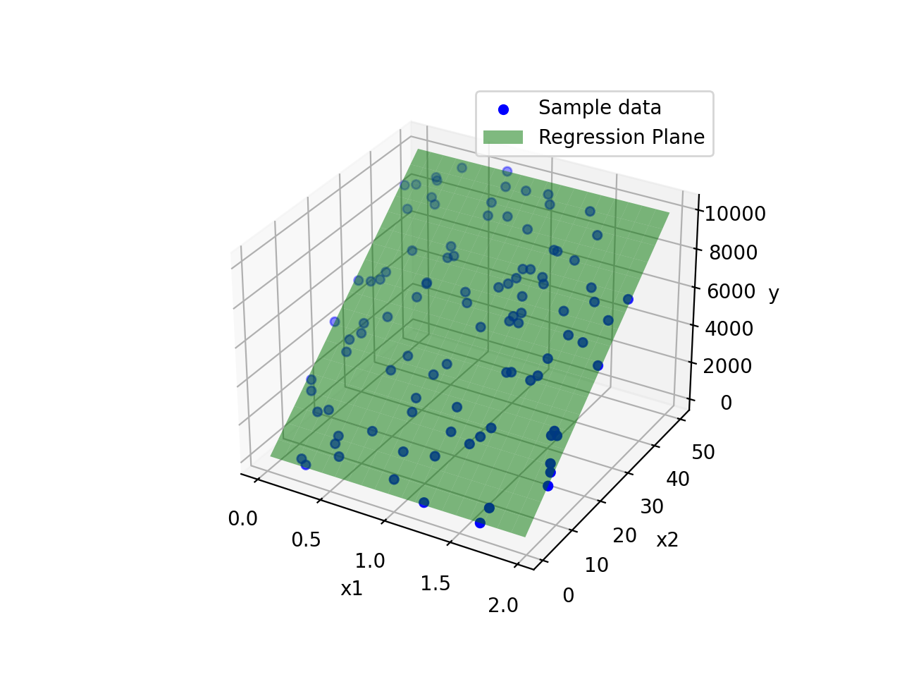
Sample data. For easier validation, I generated noisy data based a predetermined target plane ($y = 4 + 30x_1 + 200x_2$). Here, the original feature matrix $X$ is defined as $[\bold{x_1} \ \bold{x_2}]$.

Feature scaling and adding bias. To speed up the convergence, all feature columns $\bold{x_j} \in X$ were normalized to z-scores

$$\bold{x_j} := \frac{\bold{x_j} - \mu_j}{\sigma_j}$$

After that, a bias column is added:

$$\bold{X_b} := [1 \ \bold{x_1} \ ... \ \bold{x_n}]$$

Regression setup. Given the normalized feature matrix ($m$ data points) with bias column $\bold{X_b}$ and matrix of regression coefficients $\bold{\theta}=[\theta_0 \ \theta_1 \ \theta_2]^T$ ($\theta_0$ represents the bias), the regression in matrix notation is denoted as below. In numpy, all of these are np.array.

$$\bold{h_\theta}(\bold{X_b}) = \bold{X_b} \cdot \bold{\theta}$$

Loss function. The prediction error was measured through a 1/2-scaled mean square:

$$J(\bold{\theta}) = \frac{1}{2m}\sum_{i=1}^{m} (h_\theta(\bold{x^{(i)}}) - y^{(i)})^2$$

Gradient descent (regression). For each parameter $\theta_j \in \bold{\theta}$, the update through gradient descent (with learning rate $\alpha$) is defined as:

$$\theta_j := \theta_j - \alpha \frac{\partial J}{\partial \theta_j}$$

This is implemented in matrix form as:

$$\bold{\theta} := \bold{\theta} - \alpha \nabla J(\bold{\theta}) = \theta - \alpha \frac{1}{m} \bold{X_b}^T(\bold{h_\theta}(\bold{X_b}) - \bold{y})$$

Results. With $\alpha=0.01$, after 1000 iterations of gradient descent, the final parameters achieved were:

$$\theta = [5312.86566202 , 17.05242068 , 2766.87065479]$$